#R is a free statistics software
#Everything in this box is R code: Copy and past it and try it on your own!
#Everything behind a # is a comment
#Use the right arrow right to continue!
Before we can start, download and install R first:
And download and install RStudio Desktop, which is also free:

After the installation is finished, open RStudio. We will work with RStudio because it has many advantages. RStudio uses R in the background that's why we need both.
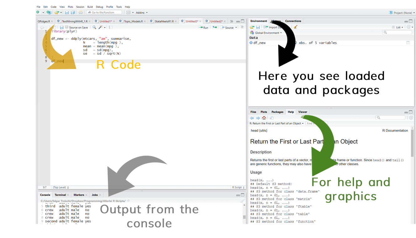
RStudio has four windows with different functions.
First steps
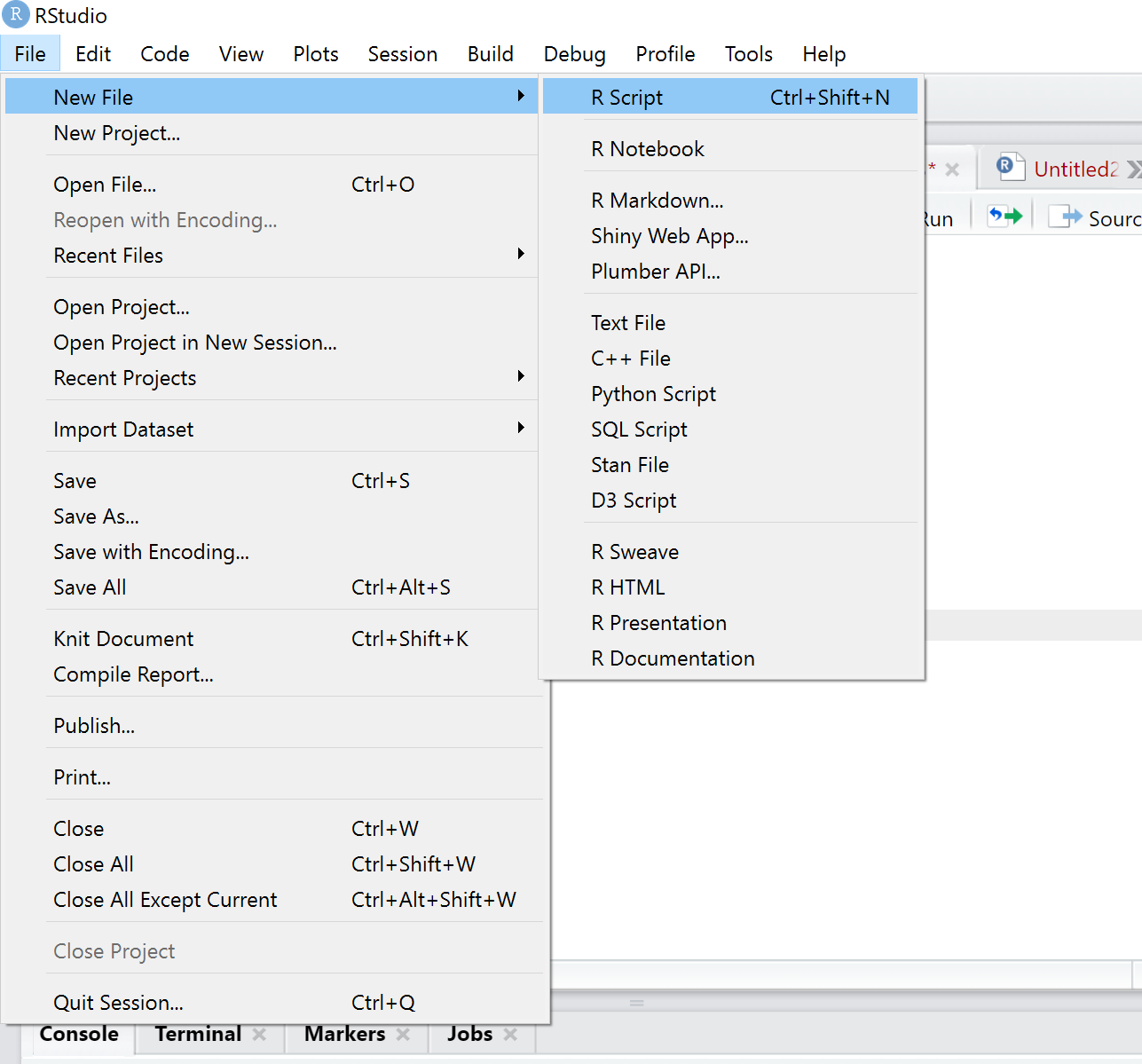
Before we can start with first calculations, please check whether the installation has worked. Please open a new R Script under File(New File). The R code will be saved in the script. It is like a do file in Stata.
Check whether your first R script is working. For example, we can use R as a calculator my typing an equation in the R script and running the code. R will solve mathematical equations for us.
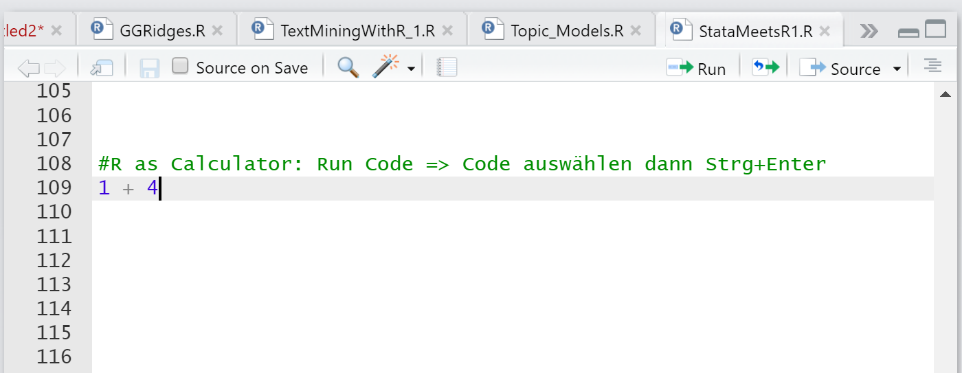
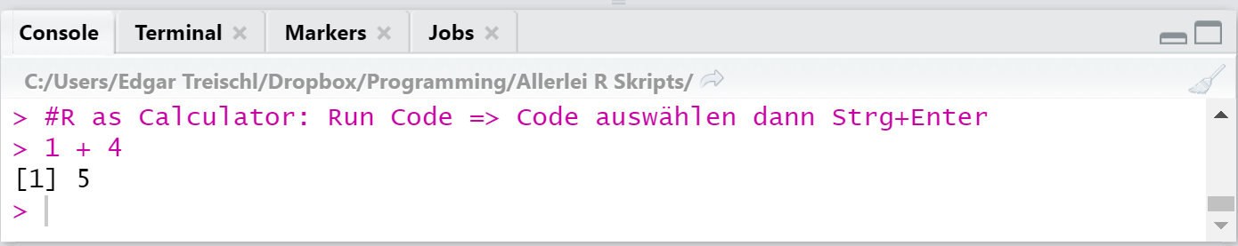
The code is being executed by pressing Ctrl + Enter. If everything works fine, you will see the following result in the output window:
Compared to Stata, R has a few special features. One of them is the assignment character "<-". The character is used to store data frames, single values and other elements in R.
# The assignment character assigns numeric values to the term before the "<-".
a <- 5
b <- 7

# You can see what's behind the saved term by calling the object again.
a
b
a + b
#Save numerical values or even complete datasets, variables and other elements as vectors with the assignment character.

b <- "Hallo World"
b
R is an open-source software, which is why many tools or packages are written by users for users. You need to install the packages and then load the corresponding library before you can use it.
#install.packages("dplyr") => installs the package dplyr
#library(dplyr) => loads the package dplyr
#These packages are already installed on my machine, that's why I put a # in front of them. Please install and load them.
On the following pages, we will repeat some core basics from Stata and I'll show you how to run the same calculations in R. We use the mtcars data set which is stored in R. If you work for the first time with a dataset, you probably want to know a few things about it before we can run some calculations.
describe
The describe command shows you stored information about the data in Stata. In R, we can display the structure of a dataset with the str() command. In addition, we have to specify the name of the dataset in the brackets.
#Stata: describe
#In R
str(mtcars)
The mtcars data contain 32 observations with information about cars, including the consumption (mpg), the number of horsepower (hp) or the transmission (am) of a vehicle.
list
The list command can be used in Stata to display single obseravation of the data, for example, as a table. In R, we can use the head() command.
#STATA: list in 1/5, table
#R: the command %>% slice(1:5) tells R that we only want to see first 5 cases like in the Stata command
head(mtcars)%>% slice(1:5)
Commands like list or head are very useful, especially to check whether the data management steps have worked.
summarize
In Stata, the summarize command calculates statistical measures of central tendencies, such as the mean or the median of the distribution. With the detail option, all measures are displayed. The summary() function in R works similar.
#STATA: summarize var, detail
#R
summary(mtcars)
#Specific variables can be selected with $variable_name.
summary(mtcars$mpg)
tab
By using the tab command you get a simple table in Stata. If you give Stata two variables names, Stata gives you a cross table in return. In R we can use the table function to produce a similar one.
#STATA: tab var1 var2
#R
table(mtcars$am,mtcars$vs)
Data preparation
Data preparation steps follow its own logic in R and it would take us an own session to learn a bit more about data preparation in R. So, let's focus first on how it works in Stata, we will see a little bit about the differences between R and Stata in another session.
Generate new variables
In Stata, a new variable can be created with generate variable and the replace command. The generate command creates a variable with missing values (.) or constant values (e.g. 1). These are placeholders and can be replaced with the if command, depending on a specified condition. For example:
#Stata:
# gen female=.
#The variable female contains first only missing values (.)
# replace female=1 if male==0
#If male equals (==) 0, the generated variable becomes 1.
# replace female=0 if male==1
#If male equals (==) 1, the generated variable becomes 0.
Recode variables
A second way to generate new variables in Stata is recode. The recode command uses an exisiting variable and recodes values of it. Important, the option gen(variable) creates a new variable, because we certainly want not to replace the original variable or values.
#Stata:
#Lets generate a new variable which indicate males in our data:
# recode female 0=1 1=0, gen (male)
#Thus, we set male now on 1, female on 0 and save it as a new variable male
#in R a new variable is added as vector <-
#recode from the dplyr package recods similar to Stata
#install and download dplyr!
#library(dplyr)
mtcars$new_var <- recode(mtcars$am, `0` = 1, `1` = 0)
mtcars%>% slice(1:5)
if conditions
In Stata, we often use if conditions for data preparation and analyses. The R universe works similar, but instead of the if condition we can use the filter() command from the dplyr package. With the help of the filter function, we can keep specific values of a variable just like the if condition. For example, we can call the filter funtion, provide R with the name of the dataframe we want to filter and then we can use mathematical operations and funtions to filter specific observations. Do you have any idea which oberservations remain in the fiter below?
#Stata: mean var if var==0
#in R:
filter(mtcars, am == 0)%>% slice(1:5)
The condition am == 0 tells R that the analysis does no longer remain on observations which meet this criteria. Or in other words, the filter only includes car with an automatic transmission (am == 0).
Load a dataset
In Stata, you can load the dataset with the use command. You have to tell Stata where to find the data by providing the file path and with the clear option you can delete all previously loaded datasets. In R, we need the package readr and the read_csv() function in order to load a csv dataframe, the rest follows the same logic. With "<-" we safe the loaded data under the name of our choice.
#library(readr) don't forget to install and load readr before running the command!
dataframe <- read_csv("C:/Users/Edgar Treischl/Desktop/titanic_R.csv")
head(dataframe)
Thanks to RStudio we don't have to remember this steps. Use RStudio to import data directly. It supports Stata, SPSS and other data formats. Let's have a look!
The button to import new data is located in the data/packages window (top right). Click on it.
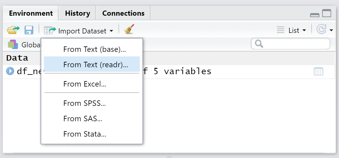
This opens the import window and you can select the new dataset.
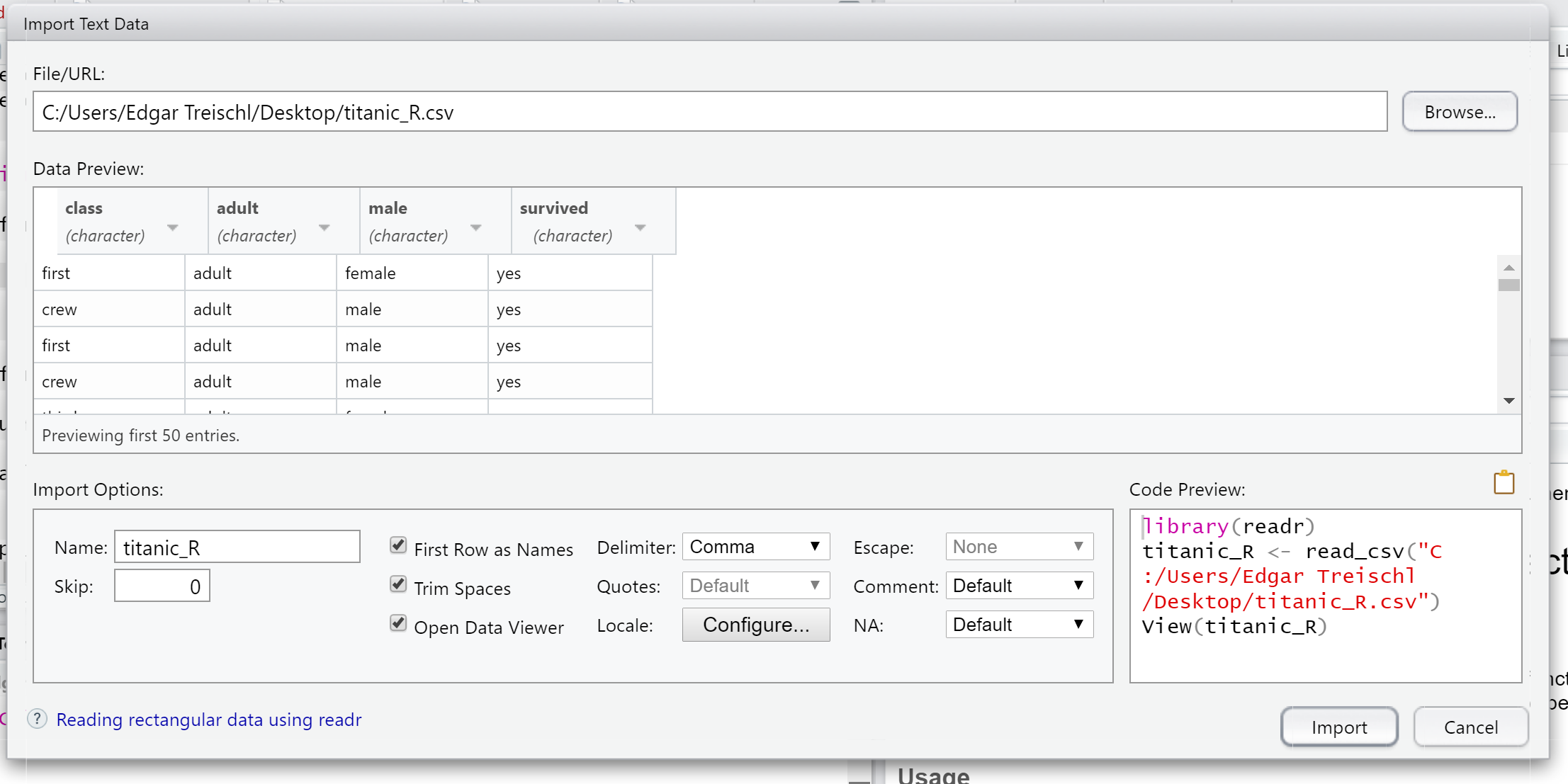
Take another look at the code preview in the right corner of the import window. After selecting the file, RStudio gives us the code and the corresponding package which is needed to load the data. Now, all you have to do is copy and paste the code to load the new dataset.
I hope this short presentation has given you an impression how the basic commands work in R. Fortunately, R has a big community and you can find many tips and tricks on the internet. Give it a try and google how you can run a linear regression in R.
# Running a multiple regression
#Let's see whether horsepower and the number of cylinders can predict mpg (miles per gallon)
fit <- lm(mpg ~ hp + cyl, data=mtcars)
summary(fit) # show results